== Indoor Localization == [[TOC(Other/Summer/2015*, depth=3)]] == Introduction == The use of GPS services is growing just as fast as the development and accessibility of mobile devices. A GPS device, which used to be a significant investment, is now included in every smartphone that emerges on the market. These services have assisted many as they navigate themselves from place to place outdoors. Although GPS is well-defined outdoors, localization indoors is still an active research problem. GPS signals indoors tend to be weaker; even if they are usable, the accuracy associated with GPS signals is not up to par. Large errors (on the order of meters) associated with GPS generally do not affect the user's ability to navigate to buildings, parks, landmarks, etc. Errors on the order of meters indoors, however, could mean that somebody is in a different room or different building altogether. A fine-grained service, down to the centimeter, is needed to localize indoors. === Motivation === An effective, low-cost, easy-to-implement solution to the indoor localization problem will have immediate impacts on everyday life, especially commercial retail. Based on movements of people in a store, retailers could determine where to place their best-selling items. They could place products effectively to accommodate shoppers and increase profits. In addition to commercial applications, indoor localization could help emergency responders efficiently respond to calls indoors, or help the elderly navigate inside a large building. Once the technology is fully developed, there are plenty of applications. === What is ORBIT Lab? === The ORBIT facility consists of a 20 x 20 grid of programmable radio nodes used to test wireless protocols and applications. Certain nodes in the facility, as well as certain sandboxes (part of the lab but not the grid), contain Universal Software Radio Peripherals (USRP), which are software defined radios that transmit and receive signals. {{{ #!html
}}} Founded in 2003 and launched in 2005, this lab provides the world's largest academic testbed for wireless communications. As of 2014, there are over 1000 registered users who have logged ~200,000 experimentation hours since the lab's founding. === Overall Approach === {{{ #!html Trilateration is the method of determining location of an object through relative distances of points and geometry of spheres. It is a method that is used in Global Positioning Systems but we intend to use the same principle in indoor localization. As illustrated below, knowing an object's relative distance from Boise, Minneapolis and Tucson, one can derive that that object is in Denver. Similarly, knowing a person's location from three USRPs enables us to roughly estimate his position in an indoor place.
}}} === Resources === '''USRP (Universal Software Radio Peripheral): '''An SDR which transmits/receives signals [[BR]] '''Wiserd: '''A spectrum sensing software used for signal processing[[BR]] '''Spectrum Analyzer: '''Device that determines signal properties at certain frequencies[[BR]] '''ESG Signal Generator: '''Device that provides reference signals in wireless connectivity[[BR]] === Procedure === Using the USRPs as both transmitters and receivers, we measure the received signal power of a certain transmitted signal and plot this measurement against the distance between the node and transmitter. We hope to obtain many distance-power measurements, which would allow us to accurately predict the the distance (but not direction) between a transmitter and receiver based on the signal power. {{{ #!html
Trilateration
The location of the transmitter and the various receivers
Experiment one: Detecting noise and signals using the nodes }}} The photos below show what occurs before the signal is transmitted and after the signal is transmitted. The ASCII art below gives us a general idea of the signal amplitude, which is then measure directly with OMF (ORBIT Management Framework) commands. {{{ #!html }}} {{{ #!html }}} {{{ #!html

Experiment two: I/Q Samples

The noise in the ORBIT lab
the signal received by a node
Analysis: The left image shows signal reception when there is no signal transmitted. This is the noise that is present while we conduct experiments in the ORBIT room. The peak that is visible in the right image is the frequency that the transmitted signal is received at the receiver nodes.
IQ samples are often used in RF applications. In signal processing, I/Q samples are the real and imaginary components of a transmitted signal. The in-phase component is the "i" and the out of phase component, shifted by 90 degrees, is "q". These samples were used to calculate the power of the signal and figure out the relationship between signal power and distance.
Real and Imaginary Signals
Verifying Reception using FFT
}}} '''Analysis:''' We used USRPs to collect the IQ samples that are portrayed in Figure 1. The graph has time on the x axis and amplitude on the y axis for both the real and imaginary components of the signal. Figure 2 verifies the reception of this signal using Fast Fourier Transform in Matlab. IQ samples are often used for modulation and demodulation of the signal that is being analyzed. We used these samples to calculate the power of the signal at known distances. {{{ #!html Experiment Three: Calculating power

Calculating signal amplitude and power is the next step in the process. The IQ samples, as mentioned above, gives the real and imaginary amplitude (y-axis) as it is related to time. Therefore, using the real amplitude on the x axis and the imaginary amplitude on the y-axis would result in the amplitude of the signal at a given time (hypotenuse). We can also calculate power from the similar calculation.
Amplitude using IQ samples
Power Program
Analysis: The figure on the left is the main principle of this power program. Using the phase, frequency and the phase angle of the sine wave, we can figure out the power of a signal by graphing the real amplitude on the x axis and the imaginary amplitude on the y axis. The hypotenuse is the amplitude of the signal. In this manner, we can figure out the power of the signal at each of the times in the domain using the program on the right. Using the average power, thereby cancelling out interference and propagation errors, we can figure out each of the powers at each distance between the receiver and the transmitter. The next step is to figure out the relationship between the two.
}}} {{{ #!html
Experiment four: Relating SNR and power to distance

Signal to noise ratio is an important part in this localization process. To maintain a high SNR at higher distances means a greater chance of better localization data since there is more signal to collect and analyze. Even in the real world, people look for gadgets and devices with a higher SNR since that provides them with greater aural experience. Due to these reasons, it is very important to analyze SNR to validate the results and conclusions of the experiments.


Signal-to-Noise ratio versus distance and the fitted curve(red)
Power vs. Distance

Analysis: Using the measured signal power, along with the distance between the transmitted and receiver, we obtained a signal amplitude-distance pair. We many of these pairs using different transmitters and receivers. We then plotted these items on a graph and found the exponential fit for the graph. As shown in this experiment, the line of best fit follows a generally negative and exponential curve but some of the points are no where close to the curve. However, the scattering of the data points signify either an error in signal processing or simply not enough data points in these graphs. We believed the latter might have had a hand in this error. }}} {{{ #!html

Experiment five: More IQ samples and updating SNR vs distance graph

As mentioned above, signal to noise ratio is very important since it relates signal quality as distance between receiver and transmitter increases. Therefore, it is important to gain points at smaller distance increments to certify that accurate data and best fit results are obtained. We obtained signal power and noise amplitude at certain distances that were not accounted before and graphed the data again.


ORBIT nodes
Updated SNR vs. Distance

Analysis: The left picture shows the board that we are using to gain our signal power and noise amplitudes during this experiment. We used one transmitter as a control and several receivers. All the "X"s in the grid are transceivers, meaning that they can be used as either a transmitter or receiver. The picture on the right is a result of the experiment. We filled in certain holes by placing the receiver and the transmitter at certain known decisions and sending signals. As seen, the curve is a better fit of the data points but there are still points that are way off the chart and the graph is still scattered. We must have more controls to figure out the problem, so we decided to test all receivers.
}}} {{{ #!html

Experiment Six: Properties of each receiver

It is possible that using each of the USRP nodes interchangeably as a transmitter or a receiver was a source of error in the experiments. Each of the nodes may have had different properties to them so they might transmit or receive signals in a completely different way. Not to mention that they might get especially awry when they are used as a transmitter at one point and then as a receiver at another. Hence the properties of each of the receivers are studied.


New Approach Board
Sandbox (Transmitter)
Analysis: Each receiver has its own characteristics. Keeping this in mind, we used a new approach (pictured on left) where we move the outdoor node(pictured on right) down the grid and receive the signals at three set receivers at known distances. Using this, we made propagation curves for each receiver to figure out how the receivers receive signals differently. After this, we can efficiently run our experiments and expect better results. Before this can be done, however, calibration of the transceivers is necessary.
}}} {{{ #!html
Experiment Seven: Transmitter Calibration

Calibration of the nodes is an important step if we are to get better localisation data and results. We have to make sure that the transmitters are transmitting the signals at the set frequency; any other frequency would offset the data. Therefore, we decided to see the difference in signal transmitting when connecting the node to a spectrum analyzer versus antenna to antenna transmission.


Wired communication
Wireless Transmission
Analysis: The left image shows the signal power that is received by transmitters connected via wire to the spectrum analyzer transmitting signals at various frequencies. As evident, they are showing a consistent (linear) increase in power as gain is increased. Conversely, the image on the right shows a rather scattered graph. This is the graph of the same transmitters transmitting via antennas, as opposed to wires. This shows that the wire transmission minimizes propagation errors while wireless transmission is prone to these errors. }}} {{{ #!html

Experiment Eight: Receiver Calibration

Calibrating the receivers is equally as important as calibrating the transmitters. The receiver was calibrated using a signal generator, a 30 dBm attenuator wire and wiserd. This calibration was to ensure that the power input and output was better hence giving us better signal power to distance data.


One GHz Power Output
Power to distance after calibration
Analysis: The left image shows the power output of the receiver at the frequency of 1 GHz. As mentioned above, the receiver was calibrated using a wire, signal generator and wiserd. The graph shows a steady increase in output beteen -110 to -60 dBm power input. Using the same carrier frequency, a signal power to distance graph was generated using the calibrated and standardized transmitter and receiver. The calibration obviously made a difference since the data points are not so scattered anymore, even when propagation is wireless, and are much closer to the theoretical free space loss model. The next step was to localize the transmitter using the data in the receivers. }}} === Plan of Action === {{{ #!html 1) Simultaneously obtain signal power values using Wiserd from all 3 receiver nodes
2) Use calibration curves to convert Wiserd values to known dBm values
3) Use propagation curves to associate dBm value with a distance
4) Insert distances into trilateration program and obtain location of transmitter }}} {{{ #!html

Results and Conclusions

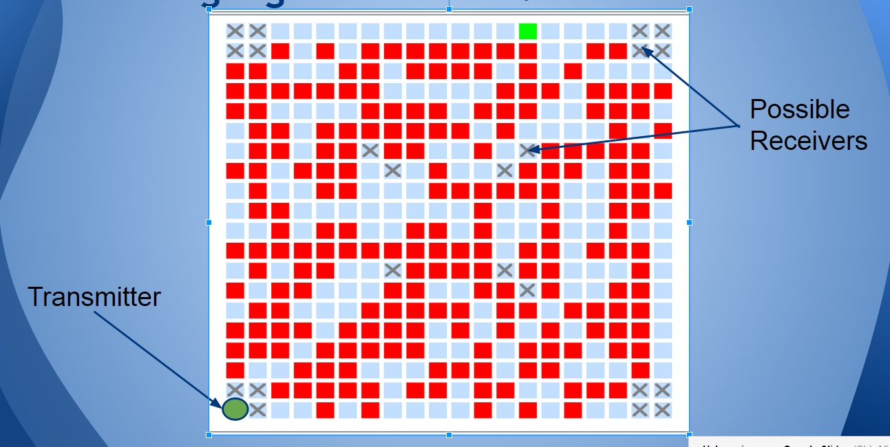
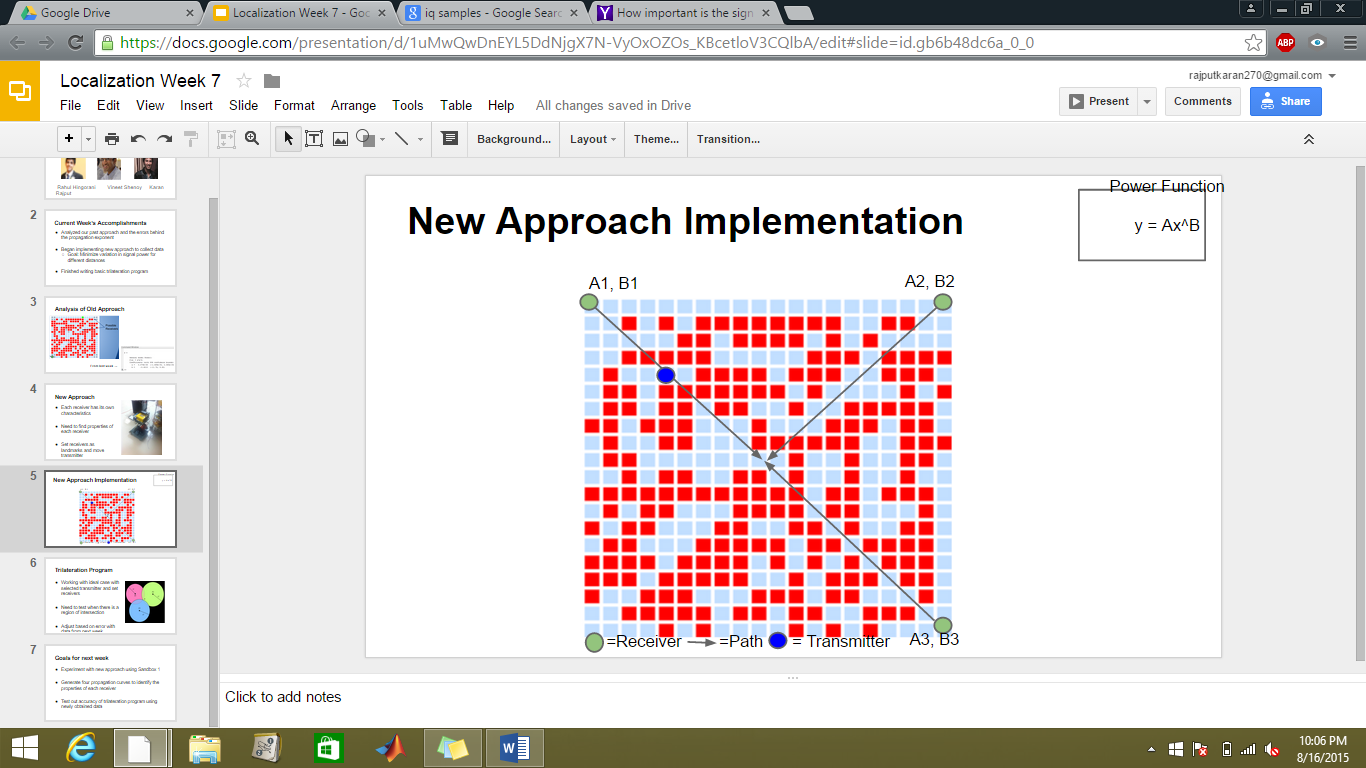
We used a trilateration program to analyze the data collected from these calibrated devices. The trilateration takes in 9 distance as inputs (3 distances from each receiver at 3 frequencies) and gives the location of the transmitter as the output. It does so but drawing three circles with the distance readings set as the radii and finds the intersection.

Our recent results have shown that if the transmitter is close to the center of the grid, the localization is most accurate. More data is necessary to come to any conclusions about accuracy of the program and results.

Transmitter Placed at (7.12, 6.4) m
Trilateration Estimate: (7.92, 8.19) m
Error: 1.75 m

Transmitter Placed at (2.25, 2.04) m
Trilateration Estimate: (5.77, 4.42) m
Error : 4.25 m

The project is no where closer to completion. Indoor localization is a topic that has been worked on for years now. For any effective method to be finalized, accurate results and collaboration are key. More work will be done on our project in the near future and updates will be posted on this page regularly.

}}} === Weekly Presentations === Presentations are done on a weekly basis before other research interns or professors. Presentations include the group's accomplishments over the past week as well as goals for the following week [https://docs.google.com/presentation/d/19tk2BQUCDE6SibGhI5q5ZbgrDVxeivjv-o5k8SRUtpU/pub?start=false&loop=false&delayms=3000 Week 2][[BR]] [https://docs.google.com/presentation/d/1bB5xOKHx_YjLfJ1QgAFkz9POWl7zakhP11L4NGwn4Mg/pub?start=false&loop=false&delayms=3000 Week 3][[BR]] [https://docs.google.com/presentation/d/1Zwrn0vNEuN4WQPvoh9i3Pk9lSppQn_kekqOq8mlOKdM/pub?start=false&loop=false&delayms=60000 Week 4][[BR]] [https://docs.google.com/presentation/d/1g_KbZgF6W24HXhJNMXTMtkahgETWTUDOlhRXyfhY3hA/pub?start=false&loop=false&delayms=3000 Week 5][[BR]] [https://docs.google.com/presentation/d/1I1gc6wtnZkyP5FN9h_qYw-3CHTYzYk9VVXQfDYBt-Ps/pub?start=false&loop=false&delayms=5000 Week 6] [[BR]] [https://docs.google.com/presentation/d/1uMwQwDnEYL5DdNjgX7N-VyOxOZOs_KBcetloV3CQlbA/pub?start=false&loop=false&delayms=5000 Week 7] [[BR]] [https://docs.google.com/presentation/d/1VErJIzLNoOnpdwJVy60t8QTDD7V3giSe0EcwfRldJS0/pub?start=false&loop=false&delayms=5000 Week 8][[BR]] [https://docs.google.com/presentation/d/1vls9I32fbq7ubQY-pouM0mt68GfNYfKto1SNjZ_iURA/pub?start=false&loop=false&delayms=5000 Week 9][[BR]] [https://docs.google.com/presentation/d/1VI2KApgiSGXkV2XYQXRTpepJmyTto9gfbUUEm6ysVs8/edit?usp=sharing Week 10][[BR]] [https://docs.google.com/presentation/d/1bl6XcSzHVppZVYgLfC7Zobgx1fosXx3bSCTkBhmmabg/edit?usp=sharing Week 11][[BR]] === Team === {{{ #!html
Rahul Hingorani
University of Michigan
Industrial/Electrical Engineering
Vineet Shenoy
Rutgers University
Electrical and Computer Engineering
Karan Rajput
Rutgers University
Electrical and Computer Engineering
}}} {{{ #!html }}}