
Table of Contents
Characterizing 5G Leakage on Passive Weather Sensing Spectrum Bands
About This Project
The goal of this Project is to determine how well a given millimeter wave frequency transmission (i.e. waveforms sent at frequencies above 20 GHz, as 5G will need to be) can stay within its allotted bandwidth. This will be accomplished by measuring the amount of "leakage" - the amount of extra energy that is present due to the transmission of a wave - at various frequencies between about 25-28 GHz. This is particularly relevant as leakage could potentially affect frequency bands used to predict weather at about 23.8 GHz. There are Experiment Reports for measuring the leakage centered at 5 GHz, as that is what much of the work during the project was accomplished with.
Background
General Background
If two signals are sent at the same frequency, they can conflict with each other. Therefore, there are spectrum licenses in each country which are earmarked for specific purposes, such as TV or phone use. Each user must stay within their allotted bandwidth (the portion of the spectrum which they own the license to) on the power-frequency plot, but as they are wave shaped, they do not naturally fit perfectly. Ideally they would appear rectangular, so as to maximize the amount of power that could be sent while staying within the intended bandwidth. In lower frequency signals, this issue is solved by having license owners designate the edges of their spectrum to be buffer zones according to FCC rules (in the United States), but this could be less effective at higher frequencies where waves will likely have a greater amount of spillover or leakage.
This issue is particularly coming to a head with the advent of 5G, which is relying on using higher frequencies to have enough spectrum. Weather prediction technology analyzes waves at about 23.8 GHz, and could be disrupted by leakage from 5G. This project aims to get a general idea about how much potential leakage there might (or might not) be.
Difficulties with the Study
- There are low level signals in the electromagnetic spectrum emanating from a variety of natural causes. This forms a "noise floor" level at frequencies across the spectrum. Transmissions (by human or natural causes) generates a jump of power (in dbm/Hz) at the frequencies which they are sent. However, this noise floor is not constant but is actually an ever changing low level wave. Therefore, calculating what value to judge as noise floor (and any amount of power above that line to be leakage above the noise floor) can be tricky.
- Licenses identify the amount of spectrum which can be used by a company/owner, within limits set by the FCC. However, it was difficult to tell in this study how to asses what should be considered spectrum within the intended bandwidth vs what is leakage.
Note about Frequencies and Bandwidth
There are multiple important values involving frequency which are relevant to this project. Center Frequency is the central frequency at which a transmission is sent and received, and tends to be where the peak of the wave is. The sampling rate (or transmission bandwidth) is the amount of spectrum/frequencies which the signal is sent at. However, the actual signal wave may be wider than this. The receiving bandwidth is the amount of spectrum analyzed by the receiver of the transmission, and is important that it is the correct width to receive the entire wave in all its width.
Weekly Progress
Week 1
- Learned how to use some initial Linux commands and access nodes (i.e. remote computers) in Orbit Lab
- Discovered how to image nodes to load a previous software setup
- Began first tutorial on sending and viewing analog waveforms with Software Defined Radios (See picture)

Week 2
- Sent analog waves of various shapes (Square, Sinusoidal, and Sawtooth), gains, sampling rates, wave frequencies, and center frequencies
- Tested hardware capabilities of a node of wave frequency vs sampling rate holding other factors constant
- Learned what WinSCP is and how to use it to get files from Orbit Lab nodes onto a personal laptop
- Figured out how to use WinSCP to transfer supplied code to a node
- Studied and adapted MATLAB code to plot waveforms in the time and frequency domains (see frequency plot below)
- Began researching OFDM (Orthogonal Frequency Division Multiplexing)

Week 3
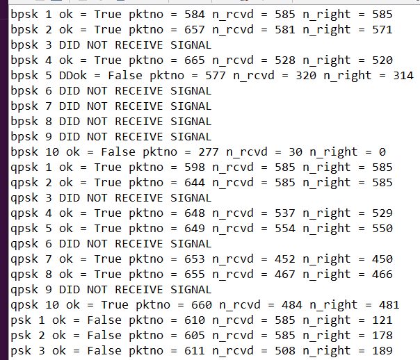
- Began sending digital waveforms with modulations (so they could actually carry information) using GNUradio and the benchmark_tx and benchmark_rx programs
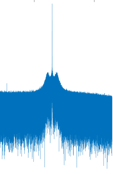
- Tested out the differences between various modulations and sampling rates using the programs rx_ascii_art_dft to see the waveforms and benchmark_rx to note the quality of the transmission (See picture)
- Found the limits of the b210 USRPs (the physical radios) at certain modulations in terms of the maximum sampling rate they could handle before underwriting (found the limits of the hardware). See picture.
- Began learning Bash to write my own scripts.

Week 4
- Wrote a bash program to simultaneously run the transmitter and receiver
- Authored another program to cycle through various modulations and sampling rates, parse the output for the final line with the results, and write that into a file
- Researched more about benchmark_tx and benchmark_rx to better understand the output
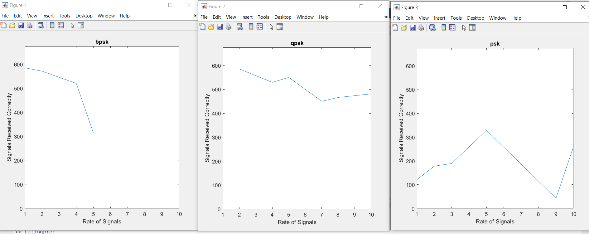
- Plotted the results in MATLab for each modulation, comparing the sampling rate of the transmission vs the number of successfully received packets of data. See picture.
- Varied other factors such as tx gain and the packet size (a total of 1Mb of data was transmitted in a number of packets, with a smaller packet size resulting in a larger number of packets, which creates more granular data)
- Began connecting to a Spectrum Analyzer

Week 5
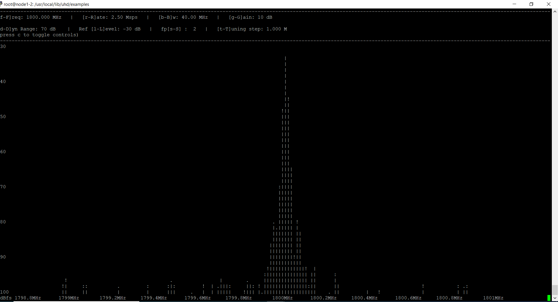
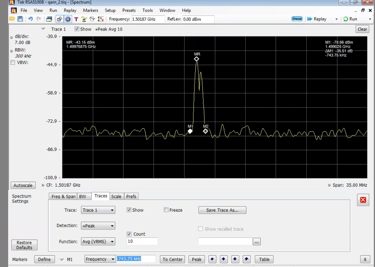
- Figured out how to see a signal on the spectrum analyzer by increasing the gain
- Researched and practiced effectively using the Spectrum Analyzer and how to save and move files onto a personal computer
- Conducted 49 tests to see the effects of varying gain and sampling rate on different modulations
- Began analyzing the spectrum analyzer's output in MATLab to find the total leakage in each waveform and plotting it vs the sampling rate for each modulation at various gains (defining the intended bandwidth to be within the -3dB bandwidth of the waveform from the peak of the signal to the peak of the noise floor)

Week 6
- Attempted to use an alternative method to determine what constitutes leakage vs intended bandwidth (using a function of the sampling rate at which the signal was sent to constitute the intended bandwidth)
- Discovered how to access the gnuradio companion (GRC) and began working on tutorials to send and receive OFDM signals.
- Wrote a few smaller programs to test out various predefined blocks
- Learned how to access the USRP radios via the GRC to get real (as opposed to simulated) data from other nodes
.png)
Week 7
- Adapted a tutorial to send and receive OFDM signals via gnuradio and the GRC
- Edited the GRC generated python code to script it so that I could have it automatically run trials given certain relevant parameters from the command line
- Wrote up a draft of Experiment 1 about my data from the trials with the spectrum analyzer (Experiment 1)
- Discovered an error on the sandbox I was using, causing me to switch to using the grid as I was planning on doing anyways (on the grid, the radios transmit waves via the air, as opposed to sandboxes where the USRP radios are connected via a wire).
Week 8
- Learned how to work with different USRPs than the version I had been using previously (N210s as opposed to B210s)
- Managed to get a connection between USRPs on the grid and download the data (and adapted the python code again so I could make it automatically run)
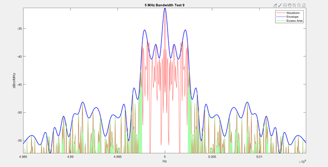
- Wrote a few MATLab codes to analyze the data files, find the envelope of the wave to find the noise floor and the -3dB bandwidth, and calculate the total area of excess bandwidth contained in the wave
- Started plotting various sampling rates vs the excess area they had in the MATLab plots (See picture).

Week 9
- Realized that the receiving bandwidth was too narrow for some of the sampling rates, causing me to set a standard for this experiment at 30 MHz
- Finished scripting/automating the data collection process (including the naming of files to include metadata about the sampling rate and other factors at which the signal was sent)
- Found a better way to account for noise by taking a sample of measurements with no signal transmission, finding the midpoint of each resulting graph, and averaging those midpoints to find the general noise level (as opposed to just assuming the edges of each graph necessarily represented the noise level).
- Took 20 samples of each sampling rate to find a more accurate plot comparing sampling rate vs excess area with a 90% margin of confidence bar
Week 10
- Wrote up Report 2 about the experiment from the previous week (Experiment 2)
- Worked to get signals using the new spectrum analyzer to get data from the millimeter wave frequencies (with a center frequency of 27GHz as opposed to previous experiments which were centered at 5GHz)
About the author(s)

This experiment was performed by Noam Hirschorn, a Rutgers University student (2023) majoring in Computer Engineering and Computer Science. The two principal advisors were Professor Ivan Seskar and Professor Narayan Mandayam. The research was conducted as part of the 2021 WINLab Summer Internship as linked below.
Attachments (11)
- Image9.png (86.2 KB ) - added by 5 years ago.
- image1.png (11.7 KB ) - added by 5 years ago.
- analog.png (97.5 KB ) - added by 5 years ago.
- benchmarkrx.png (49.2 KB ) - added by 5 years ago.
- spectrumanalyzer.png (499.5 KB ) - added by 5 years ago.
- modulplot.png (103.0 KB ) - added by 5 years ago.
- Experiment 2.docx (208.1 KB ) - added by 5 years ago.
- Experiment 1.docx (257.7 KB ) - added by 5 years ago.
- ruphoto.jpg (102.0 KB ) - added by 5 years ago.
- Screenshot (61).png (606.2 KB ) - added by 5 years ago.
- ruphoto.jpeg (69.2 KB ) - added by 5 years ago.
.png)