GNURadio

This document is not meant to be a complete tutorial on GNU Radio, but to help you start to play around GNU Radio on Orbit Sandbox and to share my experiences on exploring this wonderful toy.

Prerequisites

Before you jump into GNU Radio on Orbit, you should have a clear picture on what GNU Radio is. An excellent starting reading material is Eric Blossom’s Exploring GNU Radio:​http://www.gnu.org/software/gnuradio/doc/exploring-gnuradio.html. Eric is the founder of the whole GNU Radio project. Make sure you understand the data flow paths, including the receive path and the transmit path, understand the role that the USRP (Universal Software Radio Peripheral) plays. USRP is a flexible USB device that connects the PC to the RF world. USRP has one motherboard, which connected to the PC via USB 2.0 and can support up to four daughterboard. Each daughterboard has RF ends that can either transmit or receive waveform from the air. There are different types of daughterboard supporting a variety radio range, e.g. for example, Flex400 supports both transmit and receive in the frequency band 400MHz to 500 Mhz. You need to refresh your memory on the sample theory (Nyquist interval).

To create GNU Radio scripts, you need to build a radio by creating a graph (as in graph theory) where the vertices are signal processing blocks and the edges represent the data flow between them. The signal processing blocks are implemented in C++. The graphs are constructed and run in Python. If you are not familiar with C++ or Python, find a tutorial online and learn it.

What is Sandbox5 on Orbit-Lab?

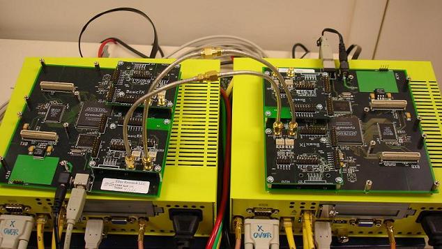
Sandbox5 consists of two nodes, i.e. node1-1 and node1-2. Each individual node is connected to one Gnuradio motherboard, and each motherboard in turn has two BasicRX and two BasicTX mounted on it, as show in the following picture.

The frequency that the BasicTX operates on ranges from 2 MHz to 200 MHz, and the BasicRX can receive from 2 MHz to 300+ MHz.

The image above shows TX_A connected to RX_B through a 50 ohm attenuator. Likewise, side B of both nodes are connected through an attenuator. The ports are connected by wires in order to minimize noise. However, both TX and RX can use actual antenna.

Setting up Sandbox 5

I assume you’ve read the tutorial about Orbit, and you know how to reserve a time slot, how to log into the nodes, and how to image the nodes. (Otherwise, read Getting Started.)

To load the nodes with the right image:

• Step 1: Login to the console.

        ssh username@ console.sb5.orbit-lab.org
  

• Step 2: Image the nodes.

        imageNodes [1,1],[1,2] gnuradio.ndz
        
        Other images are: baseline-2.1.ndz (for building from scratch, supported)
                          gnuradio_visual.ndz (for visual outputs, unsupported)
  

• Step 3: Power up node1-1 and node1-2.

        wget -O - -q 'http://cmc:5012/cmc/on?x=1&y=1'
        wget -O - -q 'http://cmc:5012/cmc/on?x=1&y=2'
  

• Step 4: Log into the node.

            ssh root@node1-1
  	  ssh root@node1-2
  

Example: Transmitting/Receiving Sine Waves

Before you run these examples, do the following:

copy ​http://www.orbit-lab.org/attachment/wiki/Documentation/GNURadio/usrp_siggen_multiple_sine.py usrp_siggen_multiple_sine.py to node1-1 (transmitter)

copy ​http://www.orbit-lab.org/attachment/wiki/Documentation/GNURadio/usrp1_rx_cfile.py usrp1_rx_cfile.py to node1-2 (receiver).

Give your scripts permission to run. (chmod +x filename)

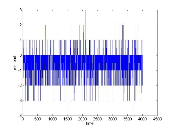
1. Receiver only The transmitter doesn't send any thing, only the receiver receives. In this case, what the receiver receives is white noise.

      ./usrp1_rx_cfile.py -f 10e3 -N21000 -g 10 noise.dat
   

   • '-f 10e3': tells the GnuRadio to listen to the frequency band centered at 10kHz.
   • '-N21000': write 21000 data points to file.
   • '-g 10': set the gain to 10.
   • 'noise.dat': set the file name that will store the data samples.

Using the matlab script ​plotall('noise.dat'), you will see the following output:

2. Transmitter and Receiver at 1MHz The transmitter sends out waveform at 1MHz, and the receiver receives at 1MHz as well. At the Transmitter node1-1:

       ./usrp_siggen_multiple_sine.py -f 1e6 -w 10k -a 1000 -m 1 --sine
   

   • '-f 1e6': tells the USRP to modulate the baseband waveform to 1MHz.
   • '—sine': the type of the waveform that will be sent out is a sine wave.
   • '-w 10k': set the original baseband frequency to 10k.
   • '-a 1000': set the amplitude to 1000.
   • '-m 1': only transmit one sine wave, instead of multiple sine waves.

At the receiver node1-2:

   ./usrp1_rx_cfile.py -f 1e6 -N21000 -g 10 rx_1m.dat

• '-f 1e6': tells the GnuRadio to listen to the frequency band centered at 1MHz.
• '-N21000': write 21000 data points to file.
• '-g 10': set the gain to 10.
• 'rx_1m.dat': set the file name that will store the data samples.

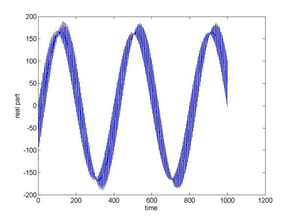
Using the matlab script ​plotall('rx_1m.dat'), you can get the following figure:

What we observe in the above plot is not a perfect sine wave. There are some high frequency components around the 10KHz sine wave. This is because that we set the target frequency as 1MHz, which is out of the working range of BasicRX and BasicTX. Recall that the working range of BasicRX and BasicTX is from 2MHz to 200MHz+. Now let’s try to set the correct frequency.

3. Transmitter and Receiver at 10MHz The transmitter sends out waveform at 10MHz, and the receiver receives at 10MHz as well. At the Transmitter node1-1:

       ./usrp_siggen_multiple_sine.py -f 10e6 -w 10k -a 1000 -m 1 --sine
   

At the receiver node1-2:

   ./usrp1_rx_cfile.py -f 10e6 -N21000 -g 10 rx_1m.dat

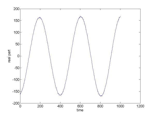
The resulting plot is :

This time the received sine wave is indeed a regular sine wave.

Note: the first 1000 data in rxXXX should be discarded. Since the receiver is starting up, the first 1000 data points are not correct.

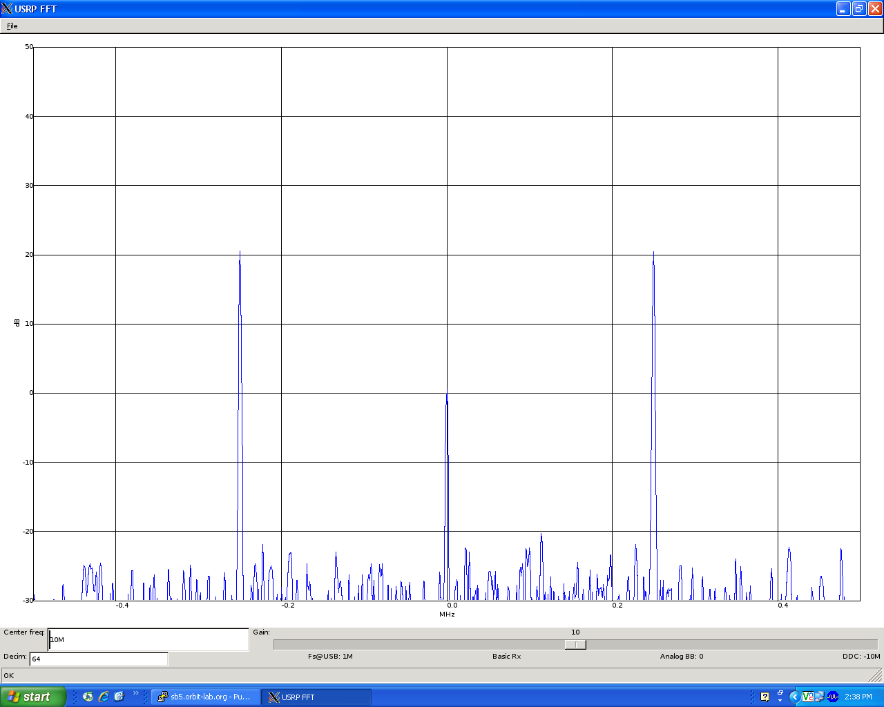
Example: Visual Outputs

Before you try these examples, you should have imaged nodes on sandbox 5 using gnuradio_visual.ndz OR manually installed x-window-system and wx-python on the node. Also be sure to have an x-server running on the local machine and make sure X is enabled on all ssh-running machines.

In the previous example, the received signal could only be viewed after it has been moved onto a machine running plotting software. With visual outputs, the researcher can analyze transmitted and received waveforms in real-time.

Some interesting visual applications included with the gnuradio software:

• usrp_fft.py — real-time fft
• usrp_oscope.py — real-time oscilloscope

Potential applications:

• Visual spectrum analyzer

Example: Audio Outputs

Even though there is no sound card on the nodes, it is still possible to listen to sounds generated by the nodes.

Troubleshooting

• Have you picked the right node as the transmitter and receiver?
• Have you run the correct Python script at the transmitter?
• Have you tune the frequency within the Radio Front’s working range?
• Have you matched the receiver’s frequency to the transmitter’s?
• Have you set the gain properly? If you fail to set the gain correctly, chances are the device will run on the saturated mode, and the result will not be pretty.

Useful Links

• The official website: ​http://www.gnu.org/software/gnuradio/index.html
• GNU Radio overview and evaluation: ​http://staff.washington.edu/~jon/gnuradio.html